
Home Cytometry History General Histories Philip Dean


The Analysis of DNA Distributions – A Brief History
by Philip Dean
In the late 1960s, a group at the Los Alamos Scientific Laboratory under the direction of Marvin Van Dilla was developing techniques to measure components in individual cells at high rates. This field was called flow cytometry and is a part of the broader field called analytical cytology. The components of interest in the cells are labeled with fluorescent dyes and the cells passed through a thin laser beam. Measurement of the light emitted by the fluorescent dyes is detected and a histogram generated of number of cells versus intensity.
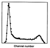
When cells in logarithmic growth were labeled with a fluorescent dye that binds specifically to DNA and measured in the flow cytometer, a DNA distribution was obtained. This distribution consists of the number of cells versus fluorescence intensity (proportional to DNA content). Figure 1 at right is a typical histogram obtained in those days.
At that time I was very interested in applying mathematical techniques and computers to biological problems. Knowing this, Van Dilla showed me one of these distributions and asked me if there was some way to obtain cell cycle parameters from the data. The biologists wanted to measure and monitor ploidy of the cells and changes in growth patterns. I told Van Dilla there must be a way to do this and agreed to look into the matter.
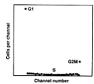
Since, if possible, mathematical models should always directly describe the biology involved, I looked up a description of the cell cycle and learned that from a DNA perspective there are three phases of the cell cycle: G1-phase in which the DNA content is constant, S-phase in which the G1 amount of DNA is doubled, and G2/M-phase in which the DNA content is constant. When a cell divides in late M-phase, the two cells produced enter G1-phase and the cycle is repeated. The biologists were interested in knowing the fraction of the cells in each phase of the cell cycle. This model of the cell cycle yields the histogram in Figure 2 at left. A perfect flow cytometer would yield such a histogram and it would be a simple matter to determine the phase fractions.
Unfortunately, flow cytometers are not perfect devices, nor is the labeling process or laser beams. Instead the type of histogram shown in Figure 1 is obtained. Certain characteristics, however, become clear. The large peak on the left represents cells in G1-phase. The peak is broad due to the imperfections in the measurement. The broadening is assumed to be represented by a normal distribution. The same is true for the peak on the right. S-phase is the problem. Its exact shape depends on the rate of DNA replication through S-phase, and this was unknown.
Since the goal was to separate the histogram into the three phases, I decided to fit it with a function consisting of two normal distributions, one for each peak, and some other function that might fit the data in S-phase. After trying a number of functions, I settled on a second degree polynomial broadened with the same variance found for the peaks. The method of least squares was used to obtain relatively unbiased results. The method chosen also yielded estimates of the errors in the computed phase fractions and a “goodness of fit.” The latter is an estimate of the quality of the overall fit to the data.
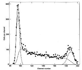
The method worked to the extent that the computed function fit the histogram data very well, as illustrated in Figure 3 at right. The dashed lines show the two fitted peaks and S-phase distributions and the solid line represents the overall fit to the data (sum of the three components). The biologists, however, wanted some independent estimate of true accuracy. At this time James Jett came to the project and took on the task of developing experiments to test the theory. He used synchronized cells and S-phase specific dyes to accomplish this. The result was that the mathematical method is quite accurate as long as the cells are in steady state growth. At this time we wrote the paper published in Cell Biology.
At this point further work was begun to develop methods of analysis for perturbed populations, both at LASL and elsewhere.
Another major use of flow cytometers was in the measurement of chromosomes. Using two fluorescent dyes, the measurement yields bivariate distributions where most of the chromosome peaks are resolved. The approach I used in this case was to describe the distribution as a series of three-dimensional normal distributions, some of which overlap. Chromosome preparations typically contained a large number of chromosome fragments. These fragments were also stained and resulted in a broad background for the chromosome peaks. In most cases I selected a paraboloid for the function, essentially a second-degree polynomial in two dimensions, sometimes adding a term to account for rotation with respect to the orthogonal axes. This analysis is much more complicated than for DNA distributions for cells, requiring six background parameters plus six parameters for each peak in the distribution. In practice, only three peaks are determined at a time. Chromosome sorting proved the validity of this method, with quite accurate results.